Oscillator Network - Oscillator Network

This Python packages contains some convenience functions to plot and generate animations of a system of coupled complex oscillators. I found some equations in a paper and I asked myself: “How do these dynamical states evolve?” So I created a small focused packaged to play with some plotting packages in Python. An example of a plot I can create with a few lines:

Loading...

This package allows static plots, plots with sliders and animations to be generated. As I am not sure I can make the slider plots possible in this static website, some plots will show here as animations.

The following Binder badge links to an interactive JupyterLab session containing some example notebooks to play around with the static plots, the dynamic plots, and the animations.

The equations¶

Equations

\begin{align} \frac{\mathrm{d}\psi_i}{\mathrm{d}t} &= \left( \gamma_i - \left| \psi_i \right|^2 \right) \psi_i + \sum_{j=1}^n J_{ij} \psi_j, \\ \frac{\mathrm{d}\gamma_i}{\mathrm{d}t} &= \varepsilon \left( 1 - \left| \psi_i \right|^2 \right). \end{align}

(1)

Where:

$t \in (0,T)$ is the time variable.
$\psi_i: (0,T) -> \mathbb{C}$ is the oscillator in site $i$ .
$\gamma_i: (0,T) -> \mathbb{R}$ is the effective injection rate of site $i$ .
$J \in \mathbb{C}^{n \times n}$ is the exchange matrix. $J_{ij}$ is the exchange constant between site $i$ and $j$ .
$\varepsilon \in \mathbb{R}$ is the responsiveness constant.

Python setup¶

import matplotlib.pyplot as plt
import numpy as np

from oscillator_network import OscillatorNetwork

# free parameters
n = 4  # number of oscillators
T = 100  # final time
Nt = 2000  # number of time steps for integration

We define a particular system:

initial_state = np.array(
    [
        -0.85831228 + 0.51312769j,
        0.9966384 + 0.08192617j,
        0.84314724 + 0.53768274j,
        0.77073359 + 0.63715754j,
    ]
)

initial_injection_rate = np.array([0.14964581, 0.69844202, 0.47997227, 0.12057254])

exchange = np.array(
    [
        [
            -0.34799573 + 0.93749612j,
            -0.99997715 + 0.00676073j,
            0.95344375 + 0.30157093j,
            -0.9773612 + 0.21157762j,
        ],
        [
            -0.16780262 + 0.98582061j,
            -0.24240459 + 0.97017525j,
            0.73768209 + 0.67514823j,
            0.85682775 + 0.51560276j,
        ],
        [
            -0.34018451 + 0.94035871j,
            -0.99982726 + 0.01858644j,
            0.46596812 + 0.88480151j,
            -0.35508116 + 0.93483548j,
        ],
        [
            0.1946992 + 0.980863j,
            -0.80616765 + 0.59168718j,
            0.88794263 + 0.45995422j,
            0.97378488 + 0.2274709j,
        ],
    ]
)

# network setup
oscnet = OscillatorNetwork(
    n=n,
    T=T,
    Nt=Nt,
    exchange=exchange,
    initial_state=initial_state,
    initial_injection_rate=initial_injection_rate,
)
oscnet

Loading...

Solving the ODEs numerically¶

This is the easy part. To solve the system, we need to use the method run():

oscnet.run()

Plots¶

Now we can plot the result in different ways.

Static plot with `matplotlib`¶

`oscillator_3d_line`¶

3D continuous plot $(\Re(\varphi_i(t)), t, \Im(\varphi_i(t)))$

fig = oscnet.plot(
    backend="matplotlib",
    figure_type="static",
    lines=["oscillator_3d_line"],
)
plt.show()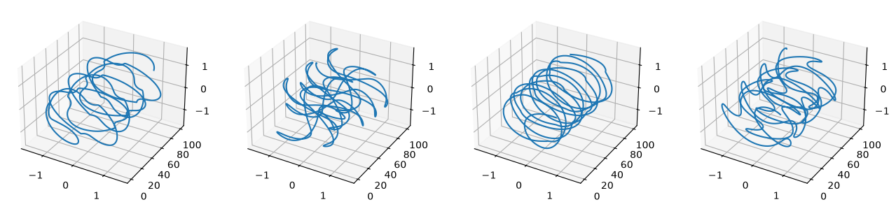

`oscillator_3d_scatter`¶

3D scatter plot $(\Re(\varphi_i(t)), t, \Im(\varphi_i(t)))$

fig = oscnet.plot(
    backend="matplotlib",
    figure_type="static",
    lines=["oscillator_3d_scatter"],
)
plt.show()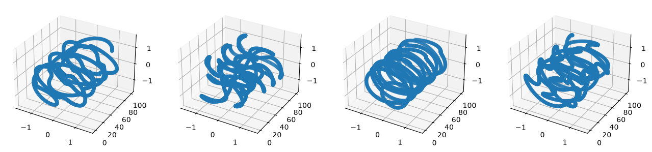

`oscillator_2d_line`¶

2d continuous plot $(\Re(\varphi_i(t)), \Im(\varphi_i(t)))$ .

fig = oscnet.plot(
    backend="matplotlib",
    figure_type="static",
    lines=["oscillator_2d_line"],
)
plt.show()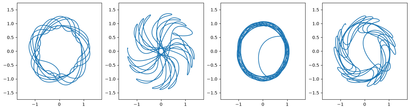

`oscillator_2d_scatter`¶

2d scatter plot $(\Re(\varphi_i(t)), \Im(\varphi_i(t)))$ .

fig = oscnet.plot(
    backend="matplotlib",
    figure_type="static",
    lines=["oscillator_2d_scatter"],
)
plt.show()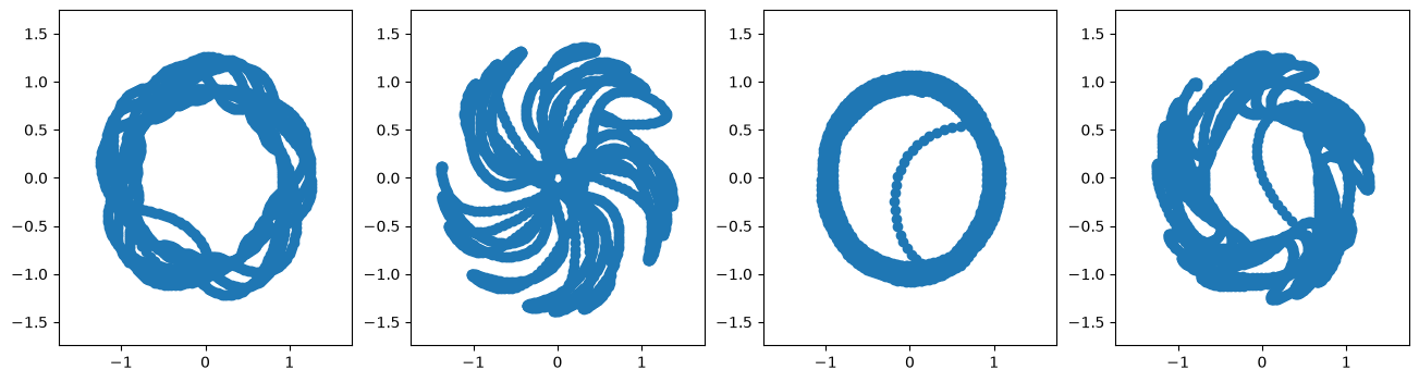

`injection_full_line`¶

Injector rate: $(t, \gamma_i(t))$

fig = oscnet.plot(
    backend="matplotlib",
    figure_type="static",
    lines=["injection_full_line"],
)
plt.show()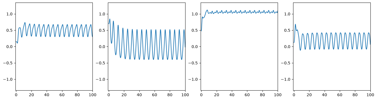

Stacking plots and including additional arguments¶

It is possible to stack in rows any of the static plots described above in a figure. The user might also want to define the list of dictionaries args for additional arguments given to each row. Each item in the list will only modify the corresponding row.

fig = oscnet.plot(
    backend="matplotlib",
    figure_type="static",
    lines=["oscillator_3d_scatter", "oscillator_2d_line", "injection_full_line"],
    args=[
        {"s": 0.5},  # size of marker for scatter point
        {"linewidth": 0.2, "color": "black"},  # width and color of line plot
        {},  # no changes for the third row
    ],
)
plt.show()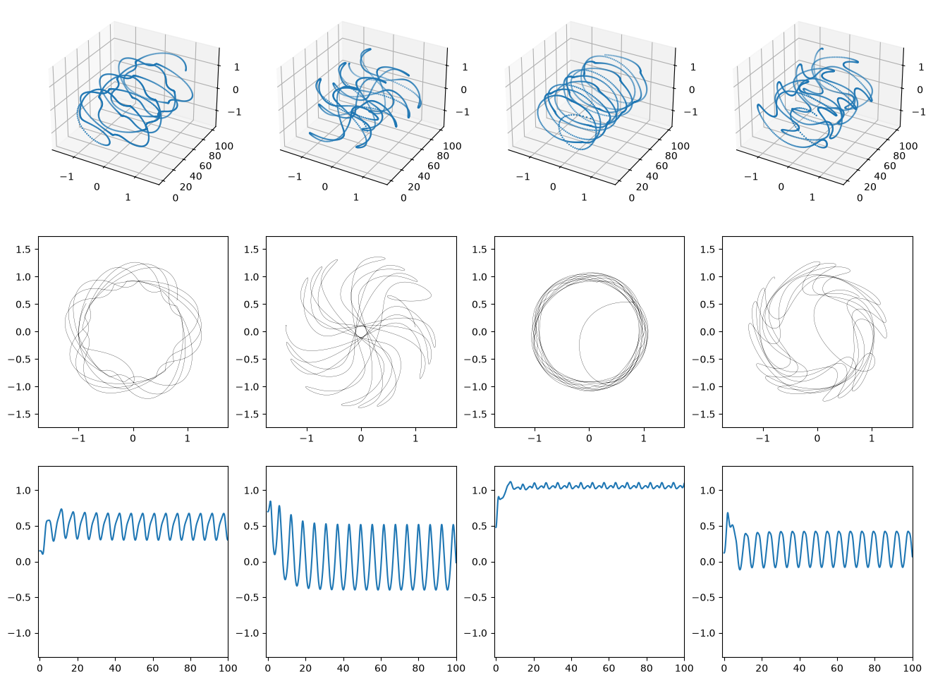

Plot with slider¶

First line: plot $(\Re(\varphi_i(t)), \Im(\varphi_i(t)))$ at each time $t$ .
Second line: $\gamma_i(t)$

%matplotlib ipympl
fig, ax, time_slider = oscnet.plot(
    backend="matplotlib",
    figure_type="slider",
    lines=["oscillator_2d_evolving"],
)
plt.show()

%matplotlib ipympl
fig, ax, time_slider = oscnet.plot(
    backend="matplotlib",
    figure_type="slider",
    lines=["oscillator_2d_evolving", "injection_full_with_mark"],
)
plt.show()

Generating animation¶

We can also generate a looping animation, and furthermore we can save it by setting save=True (warning: it can take a while).

%matplotlib ipympl
animation_time = 5  # duration of the animation in seconds
fig, ax, ani = oscnet.animation(save=False, animation_time=animation_time)

The equations¶

Python setup¶

Solving the ODEs numerically¶

Plots¶

Static plot with matplotlib¶

oscillator_3d_line¶

oscillator_3d_scatter¶

oscillator_2d_line¶

oscillator_2d_scatter¶

injection_full_line¶