Evaluate dynamics
In this notebook we show how to use the NoPEC package to evaluate the dynamics of the state variables \(y\) and \(q\).
import numpy as np

from nopec.models import FenicsModel, SparseModel
from nopec.parameters import Input, ModelParameters
from nopec.tools import initializer
Define parameters
First, we create a ModelParameters class containing all the information about the model and its discretization.
pars = ModelParameters(

    # mathematical model
    x_0=0.0,  # left point of domain
    x_L=1.0,  # right point of domain
    kappa_1=lambda x: np.ones_like(x[0]),  # diffusion function for y
    kappa_2=lambda x: np.ones_like(x[0]),  # diffusion function for q
    y_0=lambda x: 5 * np.ones_like(x[0]),  # initial value y(t=0)
    T=2.0,  # final time

    # discretization parameters
    discretization_model="fenics",  # defines the discretization model
    FE_degree=1,  # degree of finite element
    N_nodes_x=201,  # number of discretization nodes
    time_disc_met="IE",  # time discretization method (in this case Implicit Euler)
    K=201,  # number of time steps
)
pars.model_dump()
{'x_0': 0.0,
 'x_L': 1.0,
 'kappa_1': <function __main__.<lambda>(x)>,
 'kappa_2': <function __main__.<lambda>(x)>,
 'y_0': <function __main__.<lambda>(x)>,
 'T': 2.0,
 'discretization_model': 'fenics',
 'FE_degree': 1,
 'N_nodes_x': 201,
 'time_disc_met': 'IE',
 'K': 201,
 'damped_Newton': True,
 'nonlinear_conv_tol': 1e-07}
Define the input function
Models need the input function \(u\). We can use the Input to create an input array from a known function. Once chosen the one of the functions in Input, we need to evaluate it on each time step, namely \(u(t_k)\).
input_array = Input.JUMP_3_AT_166(pars.tv)
input_array
array([-3., -3., -3., -3., -3., -3., -3., -3., -3., -3., -3., -3., -3.,
       -3., -3., -3., -3., -3., -3., -3., -3., -3., -3., -3., -3., -3.,
       -3., -3., -3., -3., -3., -3., -3., -3., -3., -3., -3., -3., -3.,
       -3., -3., -3., -3., -3., -3., -3., -3., -3., -3., -3., -3., -3.,
       -3., -3., -3., -3., -3., -3., -3., -3., -3., -3., -3., -3., -3.,
       -3., -3., -3., -3., -3., -3., -3., -3., -3., -3., -3., -3., -3.,
       -3., -3., -3., -3., -3., -3., -3., -3., -3., -3., -3., -3., -3.,
       -3., -3., -3., -3., -3., -3., -3., -3., -3., -3., -3., -3., -3.,
       -3., -3., -3., -3., -3., -3., -3., -3., -3., -3., -3., -3., -3.,
       -3., -3., -3., -3., -3., -3., -3., -3., -3., -3., -3., -3., -3.,
       -3., -3., -3., -3.,  3.,  3.,  3.,  3.,  3.,  3.,  3.,  3.,  3.,
        3.,  3.,  3.,  3.,  3.,  3.,  3.,  3.,  3.,  3.,  3.,  3.,  3.,
        3.,  3.,  3.,  3.,  3.,  3.,  3.,  3.,  3.,  3.,  3.,  3.,  3.,
        3.,  3.,  3.,  3.,  3.,  3.,  3.,  3.,  3.,  3.,  3.,  3.,  3.,
        3.,  3.,  3.,  3.,  3.,  3.,  3.,  3.,  3.,  3.,  3.,  3.,  3.,
        3.,  3.,  3.,  3.,  3.,  3.])
One could as well define input_array directly as an array.
np.where(pars.tv <= 4 / 3, -3.0, +3.0)
array([-3., -3., -3., -3., -3., -3., -3., -3., -3., -3., -3., -3., -3.,
       -3., -3., -3., -3., -3., -3., -3., -3., -3., -3., -3., -3., -3.,
       -3., -3., -3., -3., -3., -3., -3., -3., -3., -3., -3., -3., -3.,
       -3., -3., -3., -3., -3., -3., -3., -3., -3., -3., -3., -3., -3.,
       -3., -3., -3., -3., -3., -3., -3., -3., -3., -3., -3., -3., -3.,
       -3., -3., -3., -3., -3., -3., -3., -3., -3., -3., -3., -3., -3.,
       -3., -3., -3., -3., -3., -3., -3., -3., -3., -3., -3., -3., -3.,
       -3., -3., -3., -3., -3., -3., -3., -3., -3., -3., -3., -3., -3.,
       -3., -3., -3., -3., -3., -3., -3., -3., -3., -3., -3., -3., -3.,
       -3., -3., -3., -3., -3., -3., -3., -3., -3., -3., -3., -3., -3.,
       -3., -3., -3., -3.,  3.,  3.,  3.,  3.,  3.,  3.,  3.,  3.,  3.,
        3.,  3.,  3.,  3.,  3.,  3.,  3.,  3.,  3.,  3.,  3.,  3.,  3.,
        3.,  3.,  3.,  3.,  3.,  3.,  3.,  3.,  3.,  3.,  3.,  3.,  3.,
        3.,  3.,  3.,  3.,  3.,  3.,  3.,  3.,  3.,  3.,  3.,  3.,  3.,
        3.,  3.,  3.,  3.,  3.,  3.,  3.,  3.,  3.,  3.,  3.,  3.,  3.,
        3.,  3.,  3.,  3.,  3.,  3.])
Model objects
Models can be initialized with a ModelParameters instance and an input_array array.
model = FenicsModel(
    pars=pars,
    input_array=input_array,
)
model
FenicsModel(input_array=array([-3., -3., -3., -3., -3., -3., -3., -3., -3., -3., -3., -3., -3.,
       -3., -3., -3., -3., -3., -3., -3., -3., -3., -3., -3., -3., -3.,
       -3., -3., -3., -3., -3., -3., -3., -3., -3., -3., -3., -3., -3.,
       -3., -3., -3., -3., -3., -3., -3., -3., -3., -3., -3., -3., -3.,
       -3., -3., -3., -3., -3., -3., -3., -3., -3., -3., -3., -3., -3.,
       -3., -3., -3., -3., -3., -3., -3., -3., -3., -3., -3., -3., -3.,
       -3., -3., -3., -3., -3., -3., -3., -3., -3., -3., -3., -3., -3.,
       -3., -3., -3., -3., -3., -3., -3., -3., -3., -3., -3., -3., -3.,
       -3., -3., -3., -3., -3., -3., -3., -3., -3., -3., -3., -3., -3.,
       -3., -3., -3., -3., -3., -3., -3., -3., -3., -3., -3., -3., -3.,
       -3., -3., -3., -3.,  3.,  3.,  3.,  3.,  3.,  3.,  3.,  3.,  3.,
        3.,  3.,  3.,  3.,  3.,  3.,  3.,  3.,  3.,  3.,  3.,  3.,  3.,
        3.,  3.,  3.,  3.,  3.,  3.,  3.,  3.,  3.,  3.,  3.,  3.,  3.,
        3.,  3.,  3.,  3.,  3.,  3.,  3.,  3.,  3.,  3.,  3.,  3.,  3.,
        3.,  3.,  3.,  3.,  3.,  3.,  3.,  3.,  3.,  3.,  3.,  3.,  3.,
        3.,  3.,  3.,  3.,  3.,  3.]), pars=ModelParameters(x_0=0.0, x_L=1.0, kappa_1=<function <lambda> at 0x7fef5bcbccc0>, kappa_2=<function <lambda> at 0x7fef5bcbcd60>, y_0=<function <lambda> at 0x7fef5bcbcc20>, T=2.0, discretization_model='fenics', FE_degree=1, N_nodes_x=201, time_disc_met='IE', K=201, damped_Newton=True, nonlinear_conv_tol=1e-07))
As the information of what discretization method is used is already present in ModelParameters.discretization_method, we can use the nopec.setup.initializer function to create the model corresponding to the requested discretization method.
initializer(pars, input_array)
FenicsModel(input_array=array([-3., -3., -3., -3., -3., -3., -3., -3., -3., -3., -3., -3., -3.,
       -3., -3., -3., -3., -3., -3., -3., -3., -3., -3., -3., -3., -3.,
       -3., -3., -3., -3., -3., -3., -3., -3., -3., -3., -3., -3., -3.,
       -3., -3., -3., -3., -3., -3., -3., -3., -3., -3., -3., -3., -3.,
       -3., -3., -3., -3., -3., -3., -3., -3., -3., -3., -3., -3., -3.,
       -3., -3., -3., -3., -3., -3., -3., -3., -3., -3., -3., -3., -3.,
       -3., -3., -3., -3., -3., -3., -3., -3., -3., -3., -3., -3., -3.,
       -3., -3., -3., -3., -3., -3., -3., -3., -3., -3., -3., -3., -3.,
       -3., -3., -3., -3., -3., -3., -3., -3., -3., -3., -3., -3., -3.,
       -3., -3., -3., -3., -3., -3., -3., -3., -3., -3., -3., -3., -3.,
       -3., -3., -3., -3.,  3.,  3.,  3.,  3.,  3.,  3.,  3.,  3.,  3.,
        3.,  3.,  3.,  3.,  3.,  3.,  3.,  3.,  3.,  3.,  3.,  3.,  3.,
        3.,  3.,  3.,  3.,  3.,  3.,  3.,  3.,  3.,  3.,  3.,  3.,  3.,
        3.,  3.,  3.,  3.,  3.,  3.,  3.,  3.,  3.,  3.,  3.,  3.,  3.,
        3.,  3.,  3.,  3.,  3.,  3.,  3.,  3.,  3.,  3.,  3.,  3.,  3.,
        3.,  3.,  3.,  3.,  3.,  3.]), pars=ModelParameters(x_0=0.0, x_L=1.0, kappa_1=<function <lambda> at 0x7fef5bcbccc0>, kappa_2=<function <lambda> at 0x7fef5bcbcd60>, y_0=<function <lambda> at 0x7fef5bcbcc20>, T=2.0, discretization_model='fenics', FE_degree=1, N_nodes_x=201, time_disc_met='IE', K=201, damped_Newton=True, nonlinear_conv_tol=1e-07))
%%time
Y_h, Q_h = model.state([3, 3, 3, 3])
CPU times: user 5.61 s, sys: 51.1 ms, total: 5.66 s
Wall time: 1.61 s
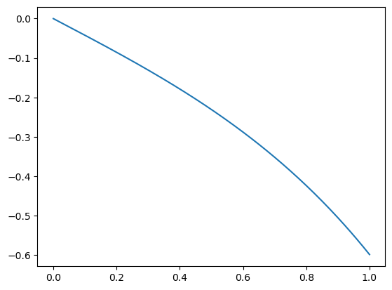
import matplotlib.pyplot as plt

plt.plot(model.FE.Omega.geometry.x[:, 0], Q_h[:, 0])
[<matplotlib.lines.Line2D at 0x7feeeb4a4050>]
Use fully discretized model
We could as well use the sparse model - fully discretized by assembling the matrices just once at the model definition.
pars.discretization_model = "sparse"
model_sparse = SparseModel(
    pars=pars,
    input_array=input_array,
)
model_sparse
SparseModel(input_array=array([-3., -3., -3., -3., -3., -3., -3., -3., -3., -3., -3., -3., -3.,
       -3., -3., -3., -3., -3., -3., -3., -3., -3., -3., -3., -3., -3.,
       -3., -3., -3., -3., -3., -3., -3., -3., -3., -3., -3., -3., -3.,
       -3., -3., -3., -3., -3., -3., -3., -3., -3., -3., -3., -3., -3.,
       -3., -3., -3., -3., -3., -3., -3., -3., -3., -3., -3., -3., -3.,
       -3., -3., -3., -3., -3., -3., -3., -3., -3., -3., -3., -3., -3.,
       -3., -3., -3., -3., -3., -3., -3., -3., -3., -3., -3., -3., -3.,
       -3., -3., -3., -3., -3., -3., -3., -3., -3., -3., -3., -3., -3.,
       -3., -3., -3., -3., -3., -3., -3., -3., -3., -3., -3., -3., -3.,
       -3., -3., -3., -3., -3., -3., -3., -3., -3., -3., -3., -3., -3.,
       -3., -3., -3., -3.,  3.,  3.,  3.,  3.,  3.,  3.,  3.,  3.,  3.,
        3.,  3.,  3.,  3.,  3.,  3.,  3.,  3.,  3.,  3.,  3.,  3.,  3.,
        3.,  3.,  3.,  3.,  3.,  3.,  3.,  3.,  3.,  3.,  3.,  3.,  3.,
        3.,  3.,  3.,  3.,  3.,  3.,  3.,  3.,  3.,  3.,  3.,  3.,  3.,
        3.,  3.,  3.,  3.,  3.,  3.,  3.,  3.,  3.,  3.,  3.,  3.,  3.,
        3.,  3.,  3.,  3.,  3.,  3.]), pars=ModelParameters(x_0=0.0, x_L=1.0, kappa_1=<function <lambda> at 0x7fef5bcbccc0>, kappa_2=<function <lambda> at 0x7fef5bcbcd60>, y_0=<function <lambda> at 0x7fef5bcbcc20>, T=2.0, discretization_model='sparse', FE_degree=1, N_nodes_x=201, time_disc_met='IE', K=201, damped_Newton=True, nonlinear_conv_tol=1e-07))
%%time
Y_h_sparse, Q_h_sparse = model_sparse.state([3, 3, 3, 3])
CPU times: user 5.73 s, sys: 7.45 ms, total: 5.74 s
Wall time: 5.76 s
import matplotlib.pyplot as plt

plt.plot(model.FE.Omega.geometry.x[:, 0], Q_h_sparse[:, 0])
[<matplotlib.lines.Line2D at 0x7feeeb374f50>]

np.linalg.norm(Y_h - Y_h_sparse), np.linalg.norm(Q_h - Q_h_sparse)
(np.float64(0.00036058486240491544), np.float64(0.0010857813921563149))